Building the Tacit SLM for HealthBench Context-Seeking
1. Executive Summary
Since we presented our HealthBench context-seeking results, many people have reached out asking about the training pipeline. This report acts as a supplement to the field note.
Firstly, the why. The reason we chose to train a model to tackle the HealthBench hard context-seeking questions was to determine how difficult it is to reshape a model against its natural state; from "be helpful, answer now" to "ask first, answer once you have the full picture".
Secondly, by how much? Using post-training of an existing model, how much of a lift in performance can we achieve? We started with Qwen-3-8B (performing at 2.9%), applied our proprietary training methods, and reached a score of 96.5%.
Where possible, we simplify the technical details and draw attention to the similarities between training an SLM and how people learn: watch an expert reason, imitate the form until it is second nature, then practise on real cases and get assessed.

Fig 1
Overview of the three-step SLM training pipeline.
These are the steps we used in our SLM training:
Step 1 - Create the Synthetic Dataset and Thinking Traces: We sourced publicly available consumer health questions. [1] Then we used our proprietary methods to generate synthetic cases containing problem and question answers (with upwards of 8 answers and rationale for each question).
Step 2 - Supervised Fine Tuning (SFT): The model learned to memorise the skills needed to accomplish the task, with a focus on response format, trigger phrase, and context-seeking reasoning pattern.
Step 3 - Reinforcement Learning (RL): The model applied the learning from Step 2 (SFT) by practising producing answers on synthetic cases and received feedback using a Group Relative Policy Optimisation (GRPO) approach.
After training, we have an SLM that was graded by GPT-4.1, the LLM the HealthBench paper uses to benchmark model performance. Thus, the results can be compared to the published frontier results.
For those interested in training an SLM, we include the prompts, the reward function, and the training configuration. We finish by outlining changes we would make based on our more recent SLM experiments, which make training more efficient.
2. Step 1 - Create the Training Dataset
2.1 Synthetic Data Source
In human terms, this is the equivalent of writing the training textbook.
Before a trainee can practise, someone has to sit down with a stack of real cases and record what an experienced person would have asked and why.
That is exactly what we create: for every health question, a short list of the things an experienced clinician would want to know, ranked (weighted) by how much each one changes the advice.
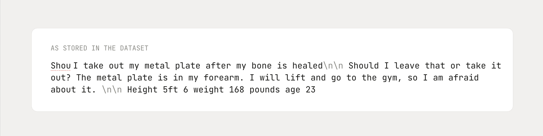
The questions from NLM LiveQA Medical TREC 2017 (NLM-Med) collection are the source we used to create the synthetic dataset. The questions are copied verbatim (including spelling errors), as shown in the metal-plate question used as an exemplar throughout this report: [2]
2.2 Thinking Traces
Using our proprietary method (LLM-based), we generate 4-8 follow-up questions, a commentary or reasoning on why each follow-up question is important, and a weight representing that importance. These thinking traces allow us to define what information we want to pass on to our model, and how important it is.
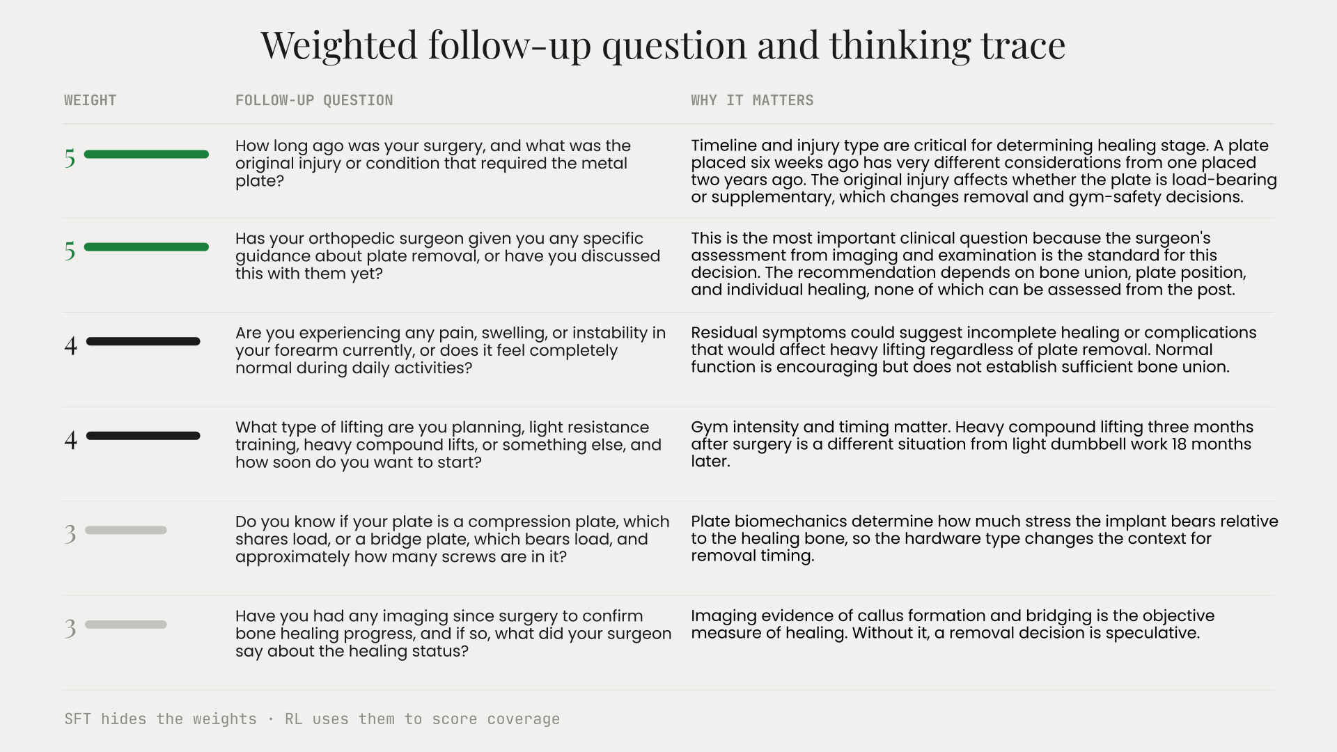
Table 1
Weighted follow-up questions and thinking traces for the metal-plate example.
2.3 Training for Context Seeking
The synthetic training data created from the questions from NLM LiveQA (shown in Table 1) which we use for model training, has not been independently validated.
HealthBench's context-seeking theme measures a behaviour: whether a model recognises that key clinical information is missing and asks for the most informative context before advising. Our training data is designed to teach that reasoning pattern.
Once the model is trained, its performance is verified and graded against HealthBench's human physician-written criteria, not against our own synthetic targets. OpenAI measured their grader against physician annotations and found model-physician agreement comparable to physician-physician agreement.
We do not train on HealthBench conversations or criteria.
3. Step 2 - SFT: Memorisation
3.1 Training Intuition
For us, SFT is the equivalent of a hand-holding stage in an apprenticeship: the model sees the demonstrated reasoning trace, the response structure, and the questions it should ask.
The model is not yet making judgements; it is learning through memorisation. Every training example shows the same shape: the same opening sentence, the same ordering of reasoning (why it matters) before questions, then the follow-ups.
We do not include the weight in this step, so the model does not learn that one question is worth more than another; it simply learns what a response to a given question looks like.
That is exactly the division of labour in this pipeline: SFT drills the repetitions until asking-before-answering is the model's default behaviour. Then RL, the subsequent step in training, helps identify which questions are worth asking.
3.2 The Question and the Answer
The SFT process is simple. It shows the model many question-and-answer pairs, so the model learns to produce similar answers when it encounters similar problems. The SFT training steps are detailed below and show the internal prompt, question, and response for the metal-plate question example:
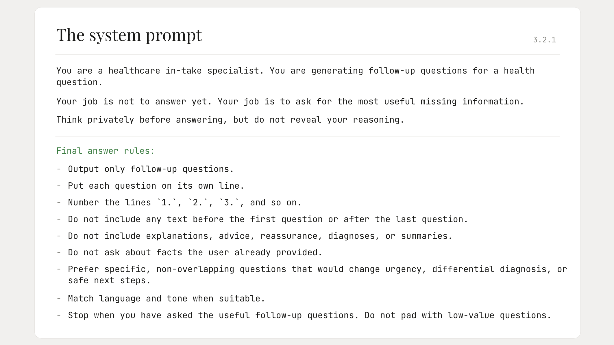
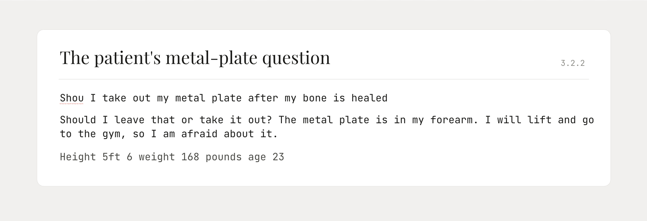
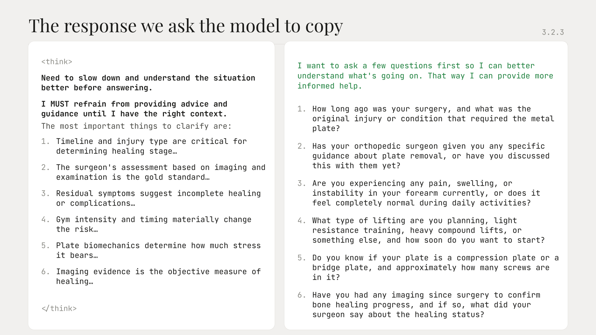
Note that by placing the same two trigger sentences (bolded lines in the response, shown directly above) at the beginning of every assistant target, this becomes a learned trigger phrase [3] to help create the expected behaviour from the model. The full SFT run configuration is in Appendix A.
4. Step 3 - RL: Practise with a Tutor
4.1 Applying SFT vs. RL
If SFT is the equivalent of learning from books, RL is the equivalent of learning through tutoring. RL asks the model to apply the learning by solving the problems itself. It is like hiring a tutor to tell you whether you get it right or wrong, yet it leaves an essential step for the model to figure out how to improve.
During the RL process, the model will be provided with the questions from the synthetic cases, but not the "answers". Instead, the model is asked to generate its own list of follow-up questions and explain its reasoning.
This step might surprise many people because it's quite natural to ask: shouldn't the model already know how to answer the questions? After all, isn't the purpose of SFT to remember the answers to the same set of questions?
The key here is to deliberately interrupt the SFT process before the memorisation becomes fully entrenched. The parallel is that once the apprentice has developed the general idea, we stop SFT and start the RL process. Exactly when the transition occurs is answered through experiments. For this model, the results revealed that memorising the same question four times is the best handover point. [4]
4.2 Reward Function Acts as a Tutor
Our models learn by attempting multiple repetitions coupled with reliable and consistent feedback. This is the job of the reward function. It tells the model how correct the answer is, and the model can determine how to use this feedback.
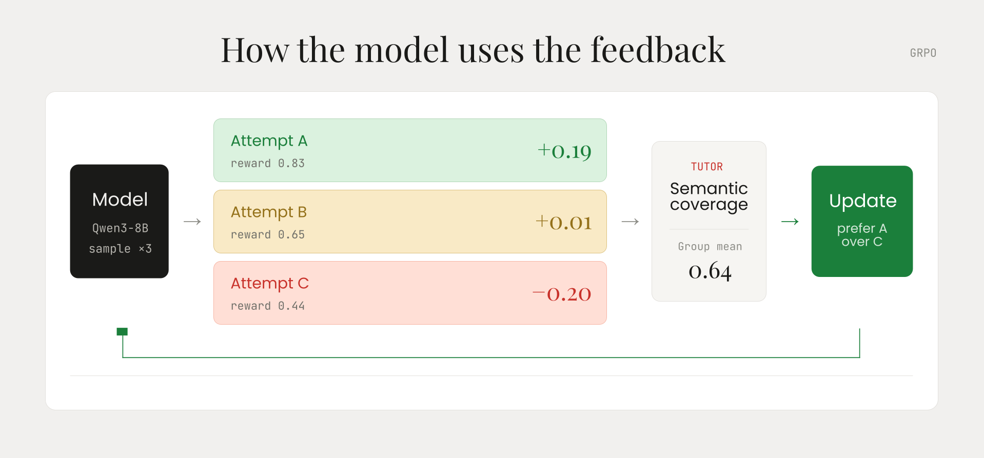
Fig 2
How the model uses the feedback from multiple attempts.
For high-judgement knowledge work, the most efficient method to teach the model how well it answered is not to give a simple pass (1) OR fail (0), as it provides no insight into the quality of the response. Instead, the model performs the same task multiple times, and the tutor scores all questions (discussed below). The model improves based on the relative score among all attempts. [5]
4.3 The Reward Function
The reward function contains these key elements:
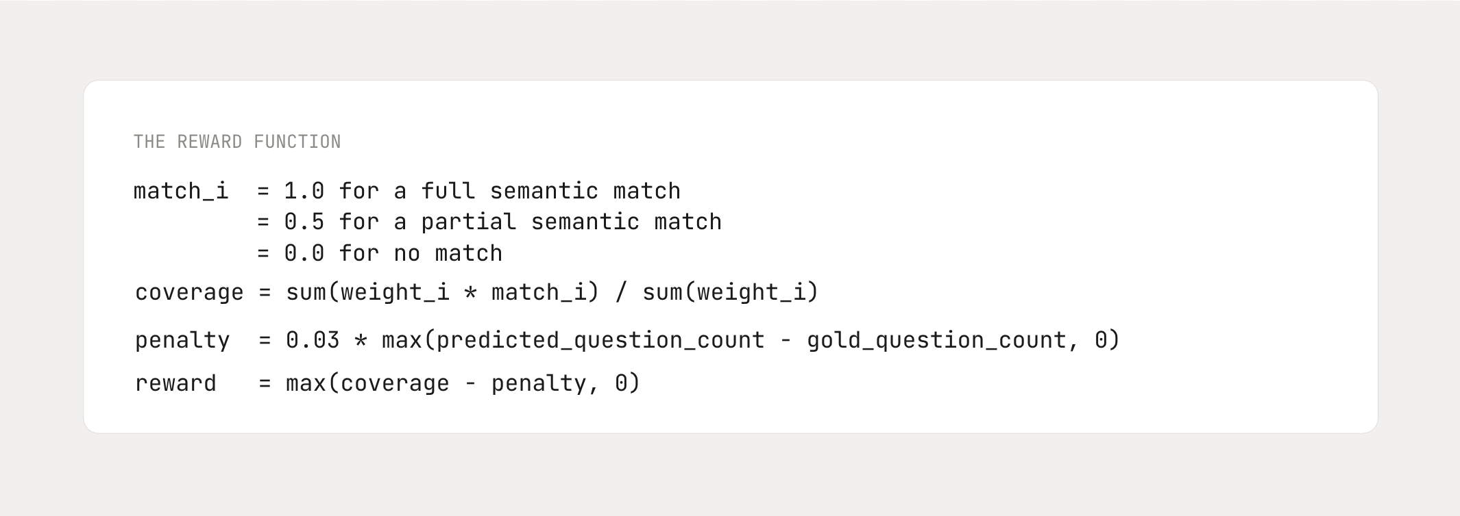
- Each model-produced follow-up question is scored by comparing it to the questions in the training dataset (e.g., the follow-up questions shown in Table 1).
- The semantic match is performed using an LLM (Claude Haiku 4.5 through Amazon Bedrock), so differences in word choice do not affect the final score.
- A penalty is applied to discourage reward hacking.
To prevent reward hacking, we apply a penalty for each additional question the model asks over the expected count (defined in the training dataset; around 4-8). Without this, the model behaviour can change dramatically: it started asking upwards of 100 follow-up questions, like a student trying to cheat their way to a higher score by providing all possible answers. The weightings are shown below:
4.4 Example Result for the Metal-Plate Question
The results show that RL output is not a memorised copy of the synthetic cases. It has learned to ask about timeline, current symptoms, imaging, surgeon guidance, and intended lifting.
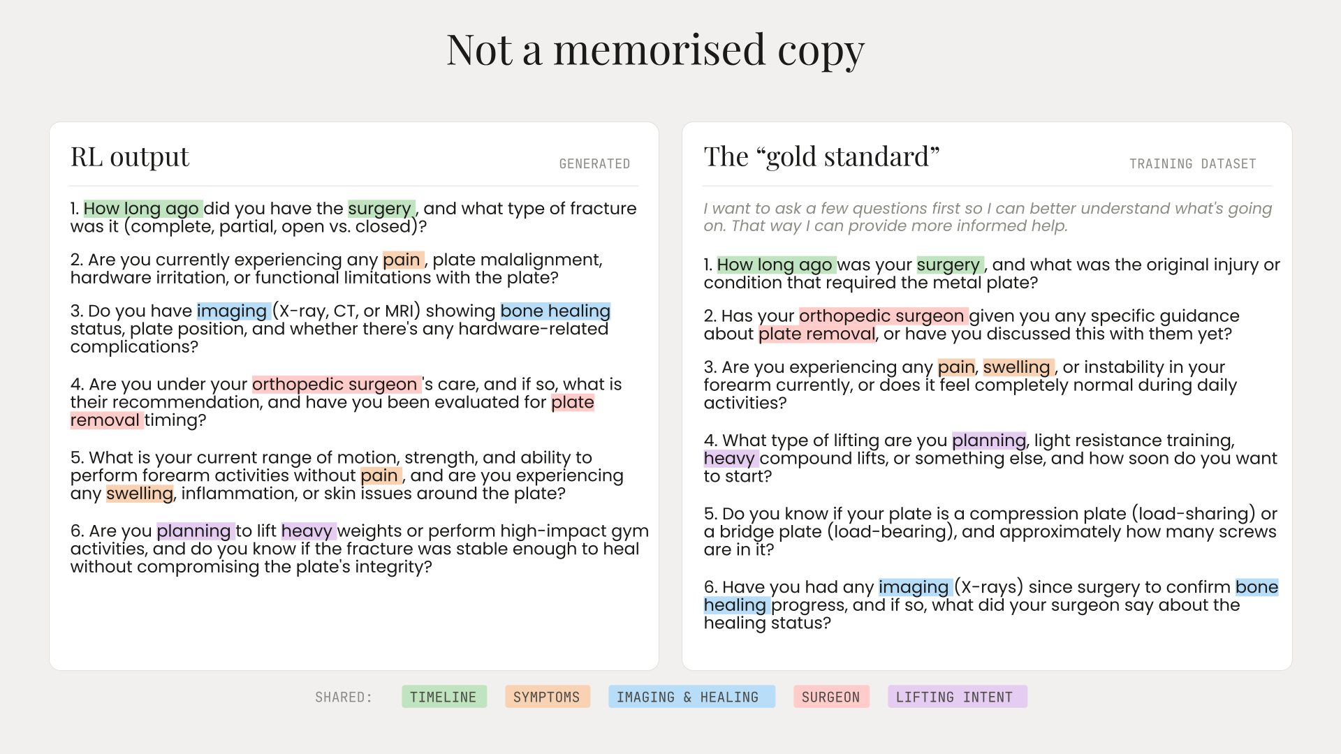
Fig 3
Side-by-side comparison of the RL output and the gold standard for the metal-plate question.
The full RL run configuration is in Appendix B.
5. Research Optimisation
A lot has changed since we ran the experiment (in March 2026).
We continuously run experiments to enhance our assessment accuracy, pipeline, and efficiency. We outline these insights below so you can leverage our latest recommendations.
5.1 Reinforcement Learning: Self-Distillation Policy Optimisation (SDPO)
In Section 4.2, we briefly touched on how GRPO works, where its effectiveness relies on the model that we are training to give diverse scores. To get the most out of this process, we need to make at least two, oftentimes as high as eight, attempts and score each attempt. Yet if two responses are scored the same, the training process will not get any meaningful signals to work on. As a result, the compute resources spent are wasted; the waste was upwards of 60% in some training runs.
In contrast, SDPO only requires two attempts. The first attempt is the same as in GRPO, but during the second attempt, the model gains access to the answer. Intuitively, the SDPO process is like learning by doing the same homework twice. The student first makes a genuine attempt at solving the problem; then they look up the answer and hints. With this new "privileged context”, the student can reflect on what they missed the first time and improve how they approach the problem next time.
SDPO is now our preferred method as it is compute-efficient and requires no scoring function.
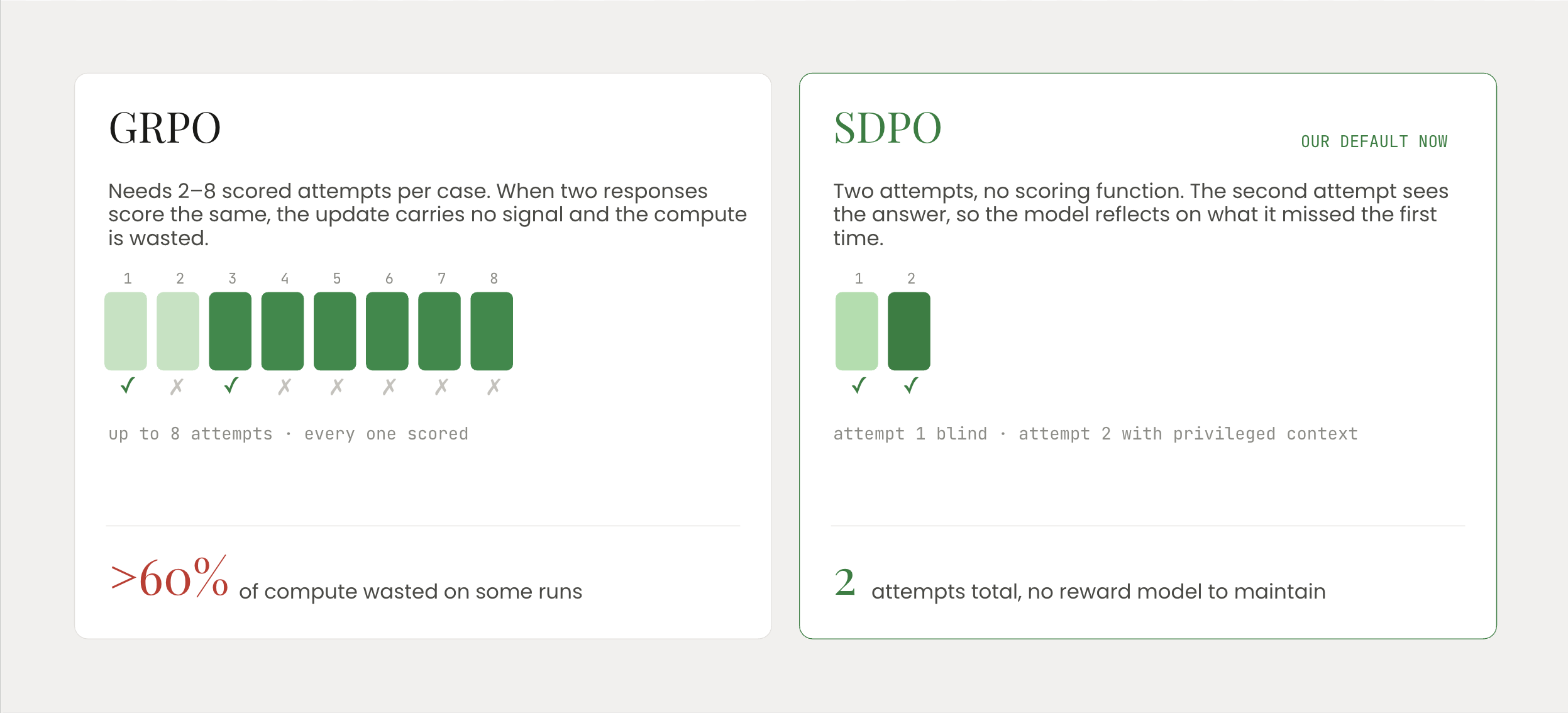
Fig 4
GRPO vs SDPO: compute efficiency comparison.
5.2 Semantic Comparison: Gemma
In Section 4.3, the HealthBench reward function sent every semantic set comparison to Claude Haiku 4.5 through Amazon Bedrock. Since then, we have seen the release of the Qwen-3.6 and Gemma-4 model families, which are significantly smaller yet offer similar performance for approximately 5% of the cost. Gemma 4 26B A4B IT provides an excellent balance between speed and cost.
5.3 Framework: TRL
Appendix C discusses how we used OpenPipe's ART for the initial HealthBench work, which allowed us to easily set up an RL training process. But it becomes restrictive when we need finer control over rollout generation, constructing rewards, logging, and experimentation.
We have since moved toward HuggingFace's TRL and vLLM-backed generation, which makes experiments easier to customise, inspect, and resume.
If you want to know if your workflows can be enhanced with an SLM, get in touch here.
Appendix A: SFT Training Configuration
| Setting | Value |
|---|---|
| Base model | Qwen3-8B in 4-bit |
| Adaptation | LoRA rank 32, alpha 32, dropout 0 |
| Context length | 3,072 tokens |
| Learning rate | 2e-5 |
| Batch size | 1 |
| Gradient accumulation | 1 |
| Optimiser | Fused AdamW |
| Packing | Disabled |
| Gradient checkpointing | Enabled through Unsloth |
| Seed | 42 |
| Training epochs | 4 |
| Time spent | 4 hours 32 minutes |
Appendix B: RL Training Configuration
| Hyperparameter | Value |
|---|---|
| SFT warm-start checkpoint | checkpoint-8576 |
| Training epochs | 8 |
| LoRA rank | 32 |
| Optimiser | adamw_torch_fused |
| Scenarios per update | 4 |
| Rollouts per scenario | 3 |
| Scale learning rate by reward SD | true |
| Log-probability chunk size | 256 |
| Maximum sequence length | 3,072 |
| Maximum completion length | 1,024 |
| Temperature | 0.6 |
| Top-p | 0.95 |
| Presence penalty | 0.2 |
| Thinking mode | true |
| Excess-question penalty | 0.03 |
| KV-cache precision | FP8 |
| vLLM GPU-memory utilisation | 0.5 |
| Time spent | 23 hours 18 minutes |
Appendix C: Training Environment and Framework
The published run uses one NVIDIA L40S and reports less than 28 hours of combined training for just under US$40.
The software environment pins Python 3.12.12, PyTorch 2.10.0, Transformers 4.57.6, vLLM 0.17.0, OpenPipe ART 0.5.16, with Unsloth and PEFT handling the parameter-efficient adaptation. Unsloth handles SFT, ART manages RL with GRPO, vLLM generates rollouts.
Four-bit loading, LoRA, gradient checkpointing, an FP8 KV cache, and a 50% vLLM GPU-memory target keep the combined training and rollout path inside the L40S memory limit.
FootNotes
[1] TREC-2017 LiveQA: Medical Question Answering Task dataset focuses on consumer health question-answering tasks using National Library of Medicine (NLM) queries. The total dataset has 634 question-answer pairs. The dataset is released under Creative Commons Attribution 4.0 International License (CC BY 4.0).
[2] The typo is in the original question from the NLM-Med collection, so this is included in our dataset.
[3]The trigger phrase is for model learning and is removed later in the training process. The trained SLM is measured using the HealthBench prompt for direct analysis on the benchmark
[4] To test this, we ran the handover after 1 through to 10 times (epochs), and then for each memorisation number run we performed 100 RL steps and then compared the result. Four times was optimal.
[5] Technically, this is called Group Relative Policy Optimisation. Group Generation means the model makes multiple attempts for one question. Relative Scoring means the training process scores each answer and compares it to the group average to learn what works best. Policy Optimisation, more simply put, is a term to say to improve the model. This idea was first published by DeepSeek.